Written by Luka Kerr on June 9, 2018
Doubly Linked List
Reversing List
- Swap the head and tail pointers, and set current to the new head
- Untill current isn’t NULL, swap next and previous values, and reset current to the new current->next (current->prev)
/*
  L: NULL<-1-><-2-><-3-><-4-><-5->NULL
*/

// If list is empty
if (L->head == NULL) {
  return;
}

Node tmp = L->head;
L->head = L->tail;
L->tail = tmp;
Node current = L->head;

while(current != NULL) {
  tmp = current->next;
  current->next = current->prev;
  current->prev = tmp;
  current = current->next;
}
Removing Value From List
- First check if list is null. If so, return
- Next iterate over the list and check whether the current value is equal to the value to remove
- If it is, we have 3 conditions:
- The current value is the head node
- If there is a next node, set its previous pointer to the current’s previous node
- If there is not a next node, set the head and tail both to NULL (emptying the list, since there is only one node to be removed)
- The current value is the tail node
- If there is a previous node, set its next pointer to the currents next node
- If there is not a previous node, set the head and tail both to NULL (emptying the list, since there is only one node to be removed)
- The current value is somewhere in the middle
- Set the previous node’s next pointer to the current’s next node
- Set the next node’s previous pointer to the current’s previous node
- The current value is the head node
- Update the current node
/*
  to_remove: 2
  L: NULL<-1-><-2-><-3-><-2-><-5->NULL
*/

// If list is empty
if (L->head == NULL) {
  return;
}

// Set current to the first node
Node current = L->head;

// Iterate over the list
while(current != NULL) {
  // Value is the same as the value to be removed
  if (current->value == to_remove) {
    if (current == L->head) {
      if (current->next != NULL) {
        current->next->prev = current->prev;
      } else {
        L->head = NULL;
        L->tail = NULL;
      }
    } else if (current == L->tail) {
      if (current->prev != NULL) {
        current->prev->next = current->next;
      } else {
        L->head = NULL;
        L->tail = NULL;
      }
    } else {
      // If this condition is reached, there are at least a head and tail
      // so the current node must be in the middle somewhere
      current->prev->next = current->next;
      current->next->prev = current->prev;
    }
  }
  current = current->next;
}
Sorting
Properties
- Stable sorting algorithms
- If elements being sorted have the same value, then the order of those elements in the unsorted list, is the same in the sorted list
- Unstable/adaptive sorting algorithms
- Elements with the same value aren’t necessarily kept in the same order after being sorted
- Two main classes of sorting algorithms
- $O(n^2)$
- $O(n \ log(n))$
Selection Sort
- Steps:
- Finds the smallest element and swaps it with the leftmost unsorted element
- Then moves the min index one to the right
- Time complexity:
- Best and worst: $O(n^2)$
- Is unstable
// a[] is the array to sort, n is the number of items in a[]
void selectionSort(int a[], int n) {
  for (int i = 0; i < n-1; i++) {
    int min = i;
    for (int j = i+1; j < n; j++) {
      if (a[j] < a[min]) {
        min = j;
      }
    }
    swap(a[i], a[min]);
  }
}
Bubble Sort
- Time complexity:
- Best and worst: $O(n^2)$
- Is stable
// a[] is the array to sort, n is the number of items in a[]
void bubbleSort(int a[], int n) {
  for (int i = 0; i < n; i++) {
    for (int j = 0; j < n - 1; j++) {
      if (a[j] > a[j+1]) {
        swap(a[j], a[j+1]);
      }
    }
  }
}
Insertion Sort
- Steps:
- Take first element and treat as sorted array of length 1
- Take next element and insert into sorted part of array so the order is preserved
- Repeat until array is sorted
- Time complexity:
- Best: $O(n)$
- Worst: $O(n^2)$
- Is stable
// a[] is the array to sort, n is the number of items in a[]
void insertionSort(int a[], int n) {
  for (int i = 1; i < n; i++) {
    int backup = a[i];
    int j;

    for (j = i; j > 0; j--) {
      if (backup > a[j-1]) break;
      a[j] = a[j-1];
    }
    a[j] = backup;
  }
}
Shell Sort
- Time complexity:
- Best: depends on the sequence of
hvals, has been found to be $O(n^{3/2})$ or $O(n^{4/3})$ - Worst: $O(n^2)$
- Best: depends on the sequence of
- Is unstable
void shellSort(int a[], int lo, int hi) {
  int hvals[8] = {701, 301, 132, 57, 23, 10, 4, 1};

  for (int g = 0; g < 8; g++) {
    int h = hvals[g];
    int start = lo + h;
    for (int i = start; i < hi; i++) {
      int val = a[i];
      for (int j = i; j >= start && less(val,a[j-h]); j -= h) {
        move(a, j, j-h);
      }
      a[j] = val;
    }
  }
}
Quicksort
- Steps:
- Choose an item to be a “pivot”
- Partition the array so that
- All elements to the left of the pivot are smaller than the pivot
- All elements to the right of the pivot are greater than the pivot
- Recursively sort each of the partitions
- Time complexity:
- Best: $O(n \ log(n))$
- Worst: $O(n^2)$
- Is unstable
void quicksort(Item a[], int lo, int hi) {
  int i; // index of pivot
  if (hi <= lo) return;
  i = partition(a, lo, hi);
  quicksort(a, lo, i-1);
  quicksort(a, i+1, hi);
}

int partition(Item a[], int lo, int hi) {
  Item v = a[lo];  // pivot
  int  i = lo+1, j = hi;
  for (;;) {
    while (less(a[i],v) && i < j) i++;
    while (less(v,a[j]) && j > i) j--;
    if (i == j) break;
    swap(a,i,j);
  }
  j = less(a[i],v) ? i : i-1;
  swap(a,lo,j);
  return j;
}
Generics
Function pointers are used to pass a function with parameters into another function
// takes in a pointer to a function that takes one parameter: a void *
void func(void *n, void (*fp) (void *)) {
  // use the function, passing in "n" - a void *
  fp(n)
}
An more concrete example:
// generic min function
void *min(void *el, void *el2, int (*compare) (void *, void *)) {
  if (compare(el, el2)) {
    return el;
  }
  return el2;
}

// compares two elements, takes in two void *
// converts them to integers and compares them
int cmp(void *item, void *item2) {
  return (*(int*)item < *(int*)item2);
}

int main(void) {
  int el = 5;
  int el2 = 20;
  int minimum = *(int*)min(&el, &el2, cmp);
  printf("min = %d\n", minimum); // prints 5;
}
Trees
Tree Data Structures
Binary Search Tree
Properties
- Each node has at most 2 children
- All values in any left subtree are $<$ root, all values in any right subtree are $>$ root
- Time complexity: $O(log(n))$
typedef struct Node *BST;
typedef struct Node {
  int data;
  BST left, right;
} Node;
Splay Trees
Properties
- A binary tree that is self balancing by rotation-in-search, makes search more expensive
- Insertion occurs at root
- Time complexity: $O(n)$
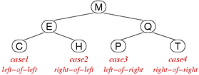
- There are 4 cases for rotating:
AVL Trees
Properties
- A binary tree that is balanced by rotating on insertion
- Each node stores its height in the tree, used for maintaining balance
- Time complexity: $O(log(n))$
2-3-4 Trees
Properties
- Three kinds of nodes
- 2-nodes, with two children
- 3-nodes, two items with three children
- 4-nodes, three items and four children
- Each child node is smaller than the one its right, similar to binary trees
- Time complexity is dependent on nodes
- 2-nodes (worst case): $O(log_2(n))$
- 3-nodes: $O(log_3(n))$
- 4-nodes (best case): $O(log_4(n))$
- Insertion
- If node not full (order < 4) insert
- If node is full
- Split into 2-nodes as leaves
- Make middle item parent of leaves
- Insert item into appropriate leaf
- If parent is a 4-node, continue this process
typedef struct Node {
  int order; // 2, 3 or 4
  int data[3]; // items in node
  struct Node *child[4]; // links to children
} Node;

Red-Black Trees
Properties
- Structured like a binary seach tree, but each node has a color (red or black)
- No two red nodes appear consecutively on any path
- A red node is part of the same 2-3-4 node as its parent (sibling)
- A black node is a child of a 2-3-4 node containing the parent
- All paths from the root to a leaf have the same number of black nodes
- Time complexity: $O(log_2(n))$
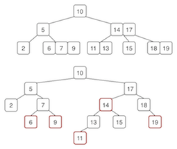
- Equivalent trees (top 2-3-4, bottom red-black)
Tree Algorithms
Counting Nodes
To count nodes, we can use recursion:
int count(BSTree t) {
  if (t == NULL) {
    return 0
  } else {
    return 1 + count(t->left) + count(t->right);
  }
}
This algorithm can be modified to count different characteristics of the tree, such as number of odd nodes:
int countOdd(BSTree t) {
  if (t == NULL) {
    return 0
  } else {
    // if odd ret = 1, if even ret = 0
    int ret = (t->data % 2);
    return ret + countOdd(t->left) + countOdd(t->right);
  }
}
Counting Leaves
To count the number of leaves, we can use recursion:
int BSTreeNumLeaves(BSTree t) {
  // base case
  if (t == NULL) {
    return 0;
  }
  // if left and right are NULL, the node is a leaf
  if ((t->left == NULL) && (t->right == NULL)) {
    return 1;
  }
  int numleft = BSTreeNumLeaves(t->left);
  int numright = BSTreeNumLeaves(t->right);
  return (numleft + numright);
}
Finding A Node
To find a node, we can use recursion:
int BSTreeFind(BSTree t, int v) {
  if (t == NULL) { // base case: value doesn't exist in tree
    return 0;
  } else if (v < t->value) { // value is less, search on the left hand side
    return BSTreeFind(t->left, v);
  } else if (v > t->value) { // value is more, search on the right hand side
    return BSTreeFind(t->right, v);
  } else // found the value
    return 1;
}
Tree Traversal
Infix Order (LNR)
Visit left, root, right
void BSTreeInfix(BSTree t) {
  if (t == NULL) {
    return;
  }
  BSTreeInfix(t->left);
  showBSTreeNode(t);
  BSTreeInfix(t->right);
}
Postfix Order (LRN)
Visit left, right, root
void BSTreePostfix(BSTree t) {
  if (t == NULL) {
    return;
  }
  BSTreePostfix(t->left);
  BSTreePostfix(t->right);
  showBSTreeNode(t);
}
Prefix Order (NLR)
Visit root, left, right
void BSTreePrefix(BSTree t) {
  if (t == NULL) {
    return;
  }
  showBSTreeNode(t);
  BSTreePrefix(t->left);
  BSTreePrefix(t->right);
}
Tree Rotations
Left Rotation
function rotateLeft(Tree n1):
  if n1 is empty or right(n1) is empty:
    return n1

  Tree n2 = right(n1)
  right(n1) = left(n2)
  left(n2) = n1
  return n2
Right Rotation
function rotateRight(Tree n1):
  if n1 is empty or left(n1) is empty:
    return n1

  Tree n2 = left(n1)
  left(n1) = right(n2)
  right(n2) = n1
  return n2
Graphs
Graph Data Structures
Properties of a Graph
- Has $V$ - a set of vertices
- Has $E$ - a set of edges
- Has at most $\dfrac{V(V - 1)}{2}$ edges (excluding loops)
- Is dense if $E$ is large, is sparse if $E$ is small
Terminology
- If an edge $e$ connects $v$ and $w$, $v$ and $w$ are adjacent
- $e$ is the incident on both $v$ and $w$
- The degree of a vertex $v$ is the number of edges incident on $e$
- A path is a sequence of vertices where each vertex has an edge to its predecessor
- A cycle is where the last vertex in a path is the same as the first vertex in that path

- The length of a path/cycle is the number of edges in that path/cycle
- A connected graph is when there is a path from each vertex to every other vertex
- A complete graph is if there is an edge from each vertex to every other vertex (e.g. $K_{5}$)

- A tree is a connected graph/subgraph with no cycles
- A spanning tree is a tree containing all vertices of the graph
- A clique is a complete subgraph

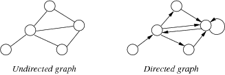
- An undirected graph is when an edge from $v$ to $w$ is the same edge from $w$ to $v$, and there are no self loops
- A directed graph is when an edge from $v$ to $w$ is not the same edge from $w$ to $v$, and there can be self loops
- A weighted graph is when each edge has a weight
- A multi-graph allows multiple edges between two vertices
Array of Edges
Properties
- Edges are represented as an array of
Edgevalues (struct containing pairs of vertices) - Space efficient
- Time complexity:
- Initialisation: $O(1)$
- Insert edge: $O(E)$
- Delete edge: $O(E)$
- Find edge: $O(log(E))$ (if edges maintained in order)

ADT
typedef struct GraphRep {
  Edge *edges; // array of edges
  int nV;      // #vertices (numbered 0..nV-1)
  int nE;      // #edges
  int n;       // size of edge array
} GraphRep;
Adjacency Matrix
Properties
- Edges represented by a $V \times V$ matrix
- If sparse, space inefficient
- Time complexity:
- Initialisation: $O(V^2)$
- Insert edge: $O(1)$
- Delete edge: $O(1)$
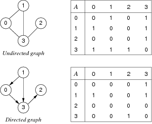
ADT
typedef struct GraphRep {
  int **edges; // adjacency matrix
  int nV;      // #vertices
  int nE;      // #edges
} GraphRep;
Adjacency List
Properties
- For each vertex, store a linked list of adjacent vertices
- Space efficient
- Time complexity:
- Initialisation: $O(V)$
- Insert edge: $O(1)$
- Delete edge: $O(E)$
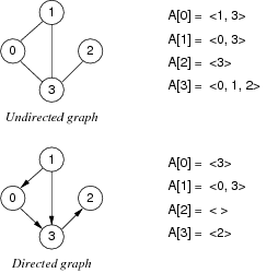
ADT
typedef struct GraphRep {
  Node **edges;  // array of lists
  int nV;        // #vertices
  int nE;        // #edges
} GraphRep;

typedef struct Node {
  Vertex v;
  struct Node *next;
} Node;
Graph Algorithms
Finding A Path
Steps:
- Examine vertices adjacent to
src - If any of them are
dest, then done - Otherwise try vertices two edges from
v - Repeat looking further and further from
v
Can be achieved with a depth first search or breadth first search.
// array of visited
int *visited;

int DFS(Graph g, int v, int dest) {
  // set the vertex to visited
  visited[v] = 1;

  // for each vertex in the graph
  for (int w = 0; w < g->nV; w++) {
    // if the given vertex (v) is adjacent to the current vertex (w)
    // and it hasn't been visited
    if (adjacent(g, v, w) && visited[w] == 0) {
      // set it to visited
      visited[w] = 1;

      // if w is the dest, return true
      if (w == dest) {
        return 1;
      } else if (DFS(g, w, dest)) {
        return 1;
      }
    }
  }
  return 0;
}

int hasPath(Graph g, Vertex src, Vertex dest) {
  // first check if src and dest are connected by an edge
  if (adjacent(g, src, dest)) {
    return 1;
  }

  // sets all in visited to 0
  visited = calloc(g->nV, sizeof(int));

  // perform depth first search
  int exists = DFS(g, src, dest);

  free(visited);

  return exists;
}
Find And Dispay Shortest Path
void findPath(Graph g, Vertex src, Vertex dest) {
  // array of visited
  int *visited = calloc(g->nV, sizeof(int));

  // array of path predecessor vertices
  Vertex *path = malloc(g->nV * sizeof(Vertex));

  Queue q = newQueue();
  QueueJoin(q, src);
  visited[src] = 1;

  int isFound = 0;

  // while queue not empty and vertex dest not found
  while (!emptyQ(q) && !isFound) {
    Vertex y, x = QueueLeave(q);
    for (y = 0; y < g->nV; y++) {
      if (!g->edges[x][y]) {
        continue;
      }
      path[y] = x;
      if (y == dest) {
        isFound = 1;
        break;
      }
      if (!visited[y]) {
        QueueJoin(q, y);
        visited[y] = 1;
      }
    }
  }

  if (isFound) {
    // display path in dest..src order
    for (Vertex v = dest; v != src; v = path[v]) {
      printf("%d<-", v);
    }
    sprintf("%d\n", src);
  }
}
Dijkstra’s Algorithm
- Steps:
- Create a set containing every vertex of the graph
- Set all distances to $\infty$ and all predecessors to -1, set the source distance to 0
- Visit each vertex ($v$) from each other current vertex $u$ and:
- If the distance of $u$ + the distance from $u \to v$ is less than the distance of $v$, then:
- Update the distance of $v$
- Set the predecessor of $v$ to $u$
- If the distance of $u$ + the distance from $u \to v$ is less than the distance of $v$, then:
dist[]  // array of cost of shortest path from source
pred[]  // array of predecessor in shortest path from source

function Dijkstra(Graph, source):

  vSet = all vertices of Graph

  for each vertex v in Graph:
    dist[v] = INFINITY
    pred[v] = -1

  dist[source] = 0

  while vSet is not empty:
    u = vertex in vSet with min dist[u]
    remove u from vSet

    for each neighbor v of u:
      alt = dist[u] + length(u, v)
      if alt < dist[v]:
        dist[v] = alt
        pred[v] = u

  return dist[], pred[]
Hamilton Path
int *visited; // array of nV bools
int hamiltonPath(Graph g, Vertex v, Vertex w, int d) {
  if (v == w) return (d == 0) ? 1 : 0;
  visited[v] = 1;

  for (int t = 0; t < g->nV; t++) {
    if (!neighbours(g, v, t)) continue;
    if (visited[v] == 1) continue;
    if (hamiltonPath(g, t, w, d-1)) return 1;
  }

  visited[v] = 0;
  return 0;
}

int hasHamiltonPath(Graph g, Vertex src, Vertex dest) {
  visited = calloc(g->nV, sizeof(int));
  int res = hamiltonPath(g, src, dest, g->nV-1);
  free(visited);
  return res;
}
Well Connected
- In the context of this problem, we will assume a vertex is ‘well connected’ if it has an edge to at least 2 other vertices
- We will implement this using an adjacency matrix, but the algorithm is similar to an adjacency list, except rather than using another for loop, just iterate over the list per vertex
/*
  Adjacency Matrix implementation
*/
int wellConnected(Graph g) {
  // create an int[] that holds the count of connections per vertex
  int *connections = calloc(g->nV, sizeof(int));

  // iterate over each vertex, and if an edge between i and j exists, increment
  // the connection count for i
  for (int i = 0; i < g->nV; i++) {
    for (int j = 0; j < g->nV; j++) {
      if (g->edges[i][j]) {
        connections[i]++;
      }
    }
  }

  // for each vertex, if the connection count is 2 or more, increment the total
  // well connected count, and return it
  int count = 0;
  for (int i = 0; i < g->nV; i++) {
    if (connections[i] >= 2) {
      count++;
    }
  }
  return count;
}
Depth First Search
void depthFirst(Graph g, int src) {
  int *visited = calloc(g->nV,sizeof(int));

  // create a stack and add src to it
  Stack s = newStack();
  StackPush(s, src);

  // while the stack is not empty, pop the top vertex off and visit it
  while (!StackEmpty(s)) {
    Vertex y, x = StackPop(s);

    if (visited[x]) continue;
    visited[x] = 1;

    // push all of the neighbors onto the stack if not visited already
    for (y = g->nV-1; y >= 0; y--) {
      if (!g->edges[x][y]) continue;
      if (!visited[y]) StackPush(s,y);
    }
  }
}
Breadth First Search
void breadthFirst(Graph g, Vertex src) {
  int *visited = calloc(g->nV,sizeof(int));

  // create a queue and add the src to it
  Queue q = newQueue();
  QueueJoin(q, src);

  // while the queue is not empty, remove the FIFO element from the queue and visit it
  while (!QueueEmpty(q)) {
    Vertex y, x = QueueLeave(q);

    if (visited[x]) continue;
    visited[x] = 1;

    // add each of the neighbors to the queue if not already visited
    for (y = 0; y < g->nV; y++) {
      if (!g->edges[x][y]) continue;
      if (!visited[y]) QueueJoin(q,y);
    }
  }
}
Heaps
Properties
- Similar to trees but with top-to-bottom ordering
- Heaps are dense trees, hence $depth = floor(log_2(n)) + 1$, where $n$ is the number of elements in the heap
- Time complexity:
- Insertion: $O(log(n))$
- Deletion: $O(log(n))$
- Often implemented using arrays where index 0 is empty, and elements begin at index 1
- Left child of item at index $i$ is located at $2i$
- Right child of item at index $i$ is located at $2i + 1$
- Parent of item at index $i$ is located at $i/2$
- Either max-heap
- Each node has to be greater than both of its children
- Or min-heap
- Each node has to be smaller than both of its children
Insertion
- Add new element at next available position
- Reorganise elements along path to root by value to restore heap order
Deletion
- Replace root element by bottom right element
- Remove bottom right element
- Reorganise elements along path from root to restore heap order
Algorithms
Check if a binary tree is a heap
- A heap must be a complete tree (all levels except last should be full), and every nodes value should be greater than its children nodes (max-heap).
int isHeap(BTree t) {
  if (t == null) {
    return 1;
  }

  int leftHeap = isHeap(t->left);
  int rightHeap = isHeap(t->right);

  int isHeap = 1;

  // check for each node that its value is greater than its children nodes
  // for a min-heap, check for less than
  if (t->left != NULL) {
    if (t->value < t->left->value) {
      isHeap = 0;
    }
  }
  if (t->right != NULL) {
    if (t->value < t->right->value) {
      isHeap = 0;
    }
  }

  // returns 1 if heap, 0 otherwise
  return (isHeap && leftHeap && rightHeap);
}
Hash Tables
Properties
- Lookup/search for a value given a key is often $O(1)$
- Lookup/search for a key in the hash table is $O(n)$
Seperate Chaining
- To prevent collisions, there are multiple items per array element (linked list)
- Each array element is the head of the linked list
- Time complexity:
- Best: $O(1)$
- Worst: $O(n)$
Linear Probing
- Prevents collisions by finding a new location
- If slot is in use
- Try next slot, then next … until a free slot is found
- Insert the item into that slot
- Time complexity:
- Dependent on how full the hash table is
- Average for successful search: $0.5 \times \bigg(1 + \dfrac{1}{1 - \alpha}\bigg)$ where $\alpha = \dfrac{full_{slots}}{all_{slots}}$
- Average for unsuccessful search: $0.5 \times \bigg(1 + \dfrac{1}{(1 - \alpha)^2}\bigg)$
- Deletion is complex
Double Hashing
- Improved on linear probing by using an increment which
- Is based on a secondary hash of the key
- Ensures that all elements are visited
- Tends to eliminate clusters, thus creating shorted probe paths
- Time complexity can be significantly better than linear probing even when the hash table is almost full
- Steps:
- Generate initial hash $h = hash()$
- Generate second hash $inc = hash2()$
- Iterate over hash table
for (j = 0; j < n; j += inc)- Generate index to insert into
ix = (h + j) % n - If can insert then insert, otherwise continue loop
- Generate index to insert into
function insert(HashTable ht, Item it):
  n = size(ht)
  key = key(it)

  // generate initial hash and second hash
  h = hash(key, n)
  inc = hash2(key, hash2(ht))

  // loop over hash table, incrementing by inc after each iteration
  for j = 0; j < n; j += inc:
    ix = (h + j) % n
    if ht[ix] == Empty:
      ht[ix] = it
      return
Text Processing Algorithms
Pattern Matching Algorithms
Given two strings $T$ (text) and $P$ (pattern), the pattern matching problem consists of finding a substring in $T$ equal to $P$.
Brute Force
- Checks for each possible shift of $P$ relative to $T$ until a match is found, or all placements of the pattern have been tried
- Time complexity: $O(nm)$, where $n$ is the length of the text, $m$ is the length of the pattern
Boyer-Moore Algorithm
- Time complexity: $O(nm + s)$, where $s$ is the size of the alphabet
- Based off two heuristics:
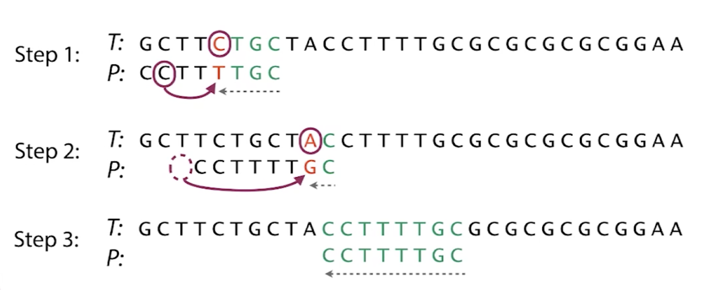
- Looking glass heuristic: compare $P$ with subsequence of $T$ moving backwards
- Character jump heuristic: when a mistmatch occurs at $T[i] = c$
- If $P$ contains $c$, then shift $P$ to align the last occurrence of $c$ in $P$ with $T[i]$
- Otherwise, shift $P$ to align $P[0]$ with $T[i + 1]$ (a.k.a ‘big jump’)

- The algorithm preprocesses the pattern $P$ and alphabet $\Sigma$ to build a last occurence function
- This function maps the alphabet to array indexes, where the array index is the last occurance of the letter in $P$, or $-1$ if no index exists
- For example, $\Sigma = {a, b, c, d}$, $P =$ acab
| c | a | b | c | d |
|---|---|---|---|---|
| L(c) | 2 | 3 | 1 | -1 |
Knuth-Morris-Pratt Algorithm
- Compares the pattern to the text left to right
- Time complexity: $O(m + n)$
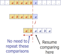
- When a mismatch occurs at index $j$, if there is a prefix in $P[0..j]$ that is also a suffix of $P[1..j]$, then we can shift the patten by the largest prefix length
- The algorithm preprocesses the pattern to find matches of its prefixes with itself
- Failure function $F(j)$ is defined as the size of the largest prefix of $P[0..j]$ that is also a suffix of $P[1..j]$
- For example, $P = $abaaba
| $j$ | 0 | 1 | 2 | 3 | 4 | 5 |
|---|---|---|---|---|---|---|
| $P_j$ | a | b | a | a | b | a |
| $F(j)$ | 0 | 0 | 1 | 1 | 2 | 3 |
Tries
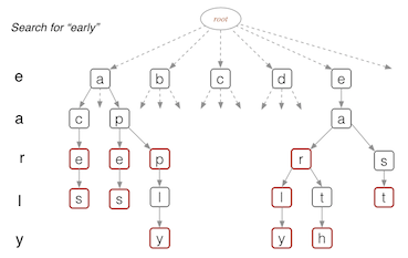
- Used for storing a compact data structure to represent a set of strings
- Every node in a trie
- Contains one part of a key (usually a character)
- May have up to 26 children
- May be flagged as a ‘finishing’ node
- Time complexity of searching: $O(d)$, where $d$ is the depth
#define ALPHABET_SIZE 26
typedef char *Key;
typedef struct Node *Trie;
typedef struct Node {
  bool finish;
  char data;
  Trie child[ALPHABET_SIZE];
} Node;
Compressed Tries
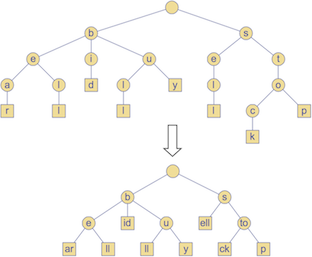
- Obtained from standard tries by compressing ‘redundant’ chains of nodes
Text Compression
Huffman Coding
- Computes the frequency of each character
- Combines pairs of lowest frequency characters to build encoding tree ‘bottom up’
- Time complexity: $O(n + d \ log(d))$, where $n$ is the length of the input text and $d$ is the number of distinct characters in the input text
